What is the formula?

First of all, Excel is, of course, a table. But tables can also be drawn in Word. The main advantage of Excel is its functions and formulas. This application is truly a powerful tool and anyone who starts using Excel sooner or later starts using formulas to solve their problems. Here I will give the basic concepts. If you know what a function is, where to find it and how to write it in a cell, then you obviously don’t need to read this section.

A function is a built-in Excel calculation tool that can return a value depending on the parameter passed to it and is intended for calculations, calculations and data analysis. Each function can include a constant, an operator, a reference, a cell name (range), and a formula.
A formula is a special Excel tool designed for calculations, calculations and data analysis. A formula can include a constant, an operator, a reference, a cell (range) name, and a function. The main difference between a formula and a function is that the formula does not have to include one of the built-in functions and can be an independent calculated expression (=12+34). In everyday use, the word most often used is formula rather than function. I don’t think this is fundamental and we need to think about it. This is already an established expression and there will clearly be no mistakes or misunderstandings on the part of others if the function is called a formula
A constant is a fixed value, which is a number or text and does not change during the calculation process.
There are three types of operators:

• Arithmetic operator– designed to perform arithmetic operations and return a numeric value;
• Comparison operator– intended for comparing data and returning the logical value TRUE or FALSE;
• Text operator– used to combine data (in Excel this is the ampersand - & ) .

Link – an indication of the cell address. Links can be absolute (that is, not changing when moving and copying a cell), relative (these links change as you move and copy the cell) and mixed. An external link is a link to a cell located in another workbook. Simply put, a cell reference is an indication of a cell or range in another formula. If you select a formula containing a reference to cells/range, different ranges and cells will be highlighted in different colors both inside the formula itself and on the sheet:

Inserting a function into a cell
You can insert a function into a cell in several ways:

To call Function Wizards you need to click the icon to the left of the formula bar: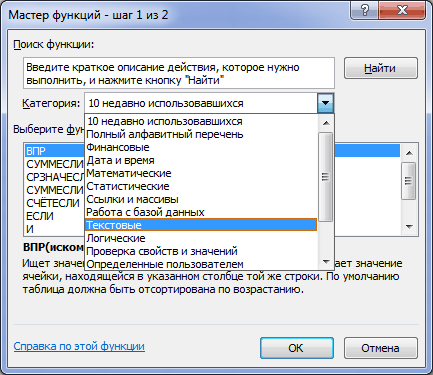


Select the category and desired function. When viewing functions, a description of the highlighted function appears at the bottom of the Function Wizard window. Through this wizard, you can view all the functions available in your version of Excel. You can also see a list of functions with descriptions on this website: Excel functions .

Entering a cell directly
If you enter an equal sign (=) in any cell and start typing the name of the function, a drop-down list will appear with all functions starting with the letters entered.

Moving through the list from the keyboard is carried out using the arrow keys, and entering a function into a cell using the key TAB. Or you can simply select the desired function with the mouse by double-clicking. After inserting the name, a hint about the arguments of the selected function will appear: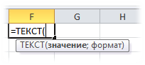

For Excel 2003 users, there is no drop-down list of functions and therefore requires the user to know the exact name of the function, because it will have to be entered completely into the memory cell. You will also have to enter all the function arguments from memory.

A function or formula must always begin with a sign = , otherwise Excel will treat what you wrote as text.

Excel will also recognize data in a cell as a formula if it begins with - or +. If text follows, Excel will return #NAME? to the cell. If numbers - Excel will try to perform mathematical operations on numbers( add, subtract, multiply, divide etc. - depending on whether the corresponding symbols are +-*/ ). But this is more an undocumented feature than a rule. It’s just that in this case, Excel itself will substitute the equality operator (=) in front of the mathematical sign, considering that it is planned to calculate something.
You can also write the function directly, starting not with the equal sign, but with the “dog” - @TDATA(). Excel itself replaces @ with =. This applies exclusively to built-in functions and is explained by backward compatibility (this type of function input was used in Lotus) so that documents created in older versions of Excel can work in later ones without loss of functionality.

Function Arguments
Almost all functions require arguments.
Argument – ​​a reference to a cell, text or number that is necessary for the function to perform calculations. For example, the function ENECHET (ISODD) requires specifying as an argument the number that needs to be checked. The result of the function will be a boolean value indicating whether the number is even or not. In this case, the argument can be specified as a number directly:
=UNCOUNT(5) – returns TRUE
=ISODD (5) – returns TRUE
So is the link to a cell containing a number:
=UNEVENT(C4) – C4 must contain a number

Or let's take the function SUM- the arguments of the function are the numbers that need to be summed. Without them, the function will not work, because... there is nothing to summarize.

If a function requires a number or text as an argument, then this can always also be a reference to a cell. If a range is required as an argument, then you must always specify a reference to a cell/range of cells
The argument separator in Russian localization is semicolon (;). In English localization it is a comma (,)
However, not all functions require mandatory input of parameters. The following functions do not have any parameters:

• TDATE()- returns the current time and date in datetime format - 01.01.2001 10:00
• TODAY()- returns the current date in date format - 01.01.2001
• TRUE() TRUE
• LIE()- returns a boolean value LIE
• ND()- returns undefined value #N/A
• PI()- returns Pi rounded to 15 digits - 3,14159265358979
• RAND()- returns a uniformly distributed random number greater than or equal to zero and less than one - 0,376514074162531

• Formulas update their result (calculate) as soon as the cell involved in the formula (influencing cell) changes its value. For example, if you write the following formula in cell A1: =D1, then when the value in cell D1 changes, it will also change in A1. A reference to cells can be not only in this form, but also as part of more complex formulas and functions, and the recalculation rule will apply to them in the same way
• Functions cannot change the values ​​and formats of other cells; they can only return the result to the cell in which they were written

Naturally, the result can be obtained using only one function, but most often various combinations of several functions are used. Using formulas you can solve many problems without resorting to help Visual Basic for Application(VBA) .

("Bottom bar":("textstyle":"static","textpositionstatic":"bottom","textautohide":true,"textpositionmarginstatic":0,"textpositiondynamic":"bottomleft","textpositionmarginleft":24," textpositionmarginright":24,"textpositionmargintop":24,"textpositionmarginbottom":24,"texteffect":"slide","texteffecteasing":"easeOutCubic","texteffectduration":600,"texteffectslidedirection":"left","texteffectslidedistance" :30,"texteffectdelay":500,"texteffectseparate":false,"texteffect1":"slide","texteffectslidedirection1":"right","texteffectslidedistance1":120,"texteffecteasing1":"easeOutCubic","texteffectduration1":600 ,"texteffectdelay1":1000,"texteffect2":"slide","texteffectslidedirection2":"right","texteffectslidedistance2":120,"texteffecteasing2":"easeOutCubic","texteffectduration2":600,"texteffectdelay2":1500," textcss":"display:block; text-align:left;","textbgcss":"display:absolute; left:0px; ; background-color:#333333; opacity:0.6; filter:alpha(opacity=60);","titlecss":"display:block; position:relative; font:bold 14px \"Lucida Sans Unicode\",\"Lucida Grande\",sans-serif,Arial; color:#fff;","descriptioncss":"display:block; position:relative; font:12px \"Lucida Sans Unicode\",\"Lucida Grande\",sans-serif,Arial; color:#fff; margin-top:8px;","buttoncss":"display:block; position:relative; margin-top:8px;","texteffectresponsive":true,"texteffectresponsivesize":640,"titlecssresponsive":"font-size:12px;","descriptioncssresponsive":"display:none !important;","buttoncssresponsive": "","addgooglefonts":false,"googlefonts":"","textleftrightpercentforstatic":40))

In this lesson we will look at how to create a complex formula in Excel, and also look at typical mistakes that novice users make due to inattention. If you have just recently been working in Excel, we recommend that you first turn to the lesson where we discussed creating simple formulas.

How to create a complex formula in Excel

In the example below, we will demonstrate how Excel calculates complex formulas based on the order of operations. In this example, we want to calculate the sales tax for food services. To do this, write the following expression in cell D4: =(D2+D3)*0.075. This formula will add up the cost of all invoice items and then multiply by the sales tax amount 7,5% (written as 0.075).

Excel follows this order and adds the values ​​in parentheses first: (44.85+39.90)=$84.75 . Then multiplies this number by the tax rate: $84.75*0.075 . The result of the calculation shows that the sales tax will be $6.36 .

It is extremely important to enter complex formulas in the correct order. Otherwise, Excel calculations may be inaccurate. In our case, if there are no parentheses, the multiplication is performed first and the result will be incorrect. Parentheses are the best way to define the order of calculations in Excel.

Create complex formulas using workflow

In the example below, we'll use links along with quantitative data to create a complex formula that will calculate the total cost of a food bill. The formula will calculate the cost of each menu item and then add all the values ​​together.

You can add parentheses to any formula to make it easier to understand. Although this will not change the result of the calculation in this example, we can still enclose the multiplication in parentheses. This will clarify that it is performed before addition.

Excel does not always warn you about errors in a formula, so you need to check all your formulas yourself. To learn how to do this, check out the lesson Checking Formulas.

Excel, unlike Word, allows you to create tables that are almost unlimited in size, but this is still not the biggest advantage of spreadsheets. The main thing is the ability to automate calculations, especially multiple ones. These can be monthly or quarterly calculations, or calculations in which you need to “play” with the source data. To automate calculations, the table must have formulas. About the techniques creating formulas in spreadsheets you can learn from this article.

Think back a little about elementary school and arithmetic. On an Excel sheet, first create a table with the original numbers.

To paste formula to add, do several steps:

• click on cell, where it should be displayed result(in the figure this is cell D2);
• enter sign = (this is a mandatory condition, otherwise the program will not distinguish the formula from everything else);
• click on the first number (in the picture it is cell A2);
• enter sign + ;
• click on the second number (in the picture it is cell AT 2);
• press the key ENTER(completion of input).

After completing the input, the formula is no longer visible in cell D2, but the result is visible. After some time, you may forget where the formulas were and where the numbers were. Will remind you of this data entry line, where you can always see what is actually in the cell, you just need to click on this cell.

Cell addresses in formulas can be written manually using the keyboard, but then you need to remember to make sure that the English language is turned on, otherwise you risk seeing a message instead of the result #NAME?.

A logical question: why not create a formula using numbers, since the result is the same?

The fact is that in this case, when changing the first or second number, or both of them, an automatic recalculation will not occur, as in the case of using cell addresses.

To create formulas for performing other actions, follow the same steps as for addition, just use the appropriate signs.

If you need to specify calculations in a formula that violate priority operations, then use brackets.

Often you need to perform the same operations on data from multiple columns. In this case, you do not need to create a new formula for each line; one is enough. Then move your mouse over marker V cell corner and drag down (use the same technique if the same calculations are performed on data from two lines, just drag the marker to the left or right - depending on the situation).

Excel is a smart program; when you drag the formula down, the line numbers in the cell addresses will automatically change, and when you drag it to the side, the letters of the columns will change.

There are tasks when the address of one cell must change when copying a formula, but not another, or only one part of it can be changed: only a letter or only a number. Then before any element that should not change, put the sign $ .

A formula is an expression that calculates the value of a cell. Functions are predefined formulas and are already built into Excel.

For example, in the figure below the cell A3 contains a formula that adds cell values A2 And A1.

One more example. Cell A3 contains a function SUM(SUM), which calculates the sum of the range A1:A2.

SUM(A1:A2)
=SUM(A1:A2)

Entering a formula

To enter the formula, follow the instructions below:

Advice: Instead of manually typing A1 And A2, just click on the cells A1 And A2.

Editing Formulas

When you select a cell, Excel displays the value or formula in the cell in the Formula Bar.

1. 1. To edit a formula, click on the formula bar and change the formula.

Operation priority

Excel uses a built-in order in which calculations are carried out. If part of the formula is in parentheses, it will be calculated first. Then multiplication or division is performed. Excel will then add and subtract. See example below:

First Excel multiplies ( A1*A2), then adds the cell value A3 to this result.

Another example:

Excel first calculates the value in parentheses ( A2+A3), then multiplies the result by the cell size A1.

Copy/paste formula

When you copy a formula, Excel automatically adjusts the references for each new cell the formula is copied into. To understand this, follow these steps:

Inserting a function

All functions have the same structure. For example:

SUM(A1:A4)
SUM(A1:A4)

The name of this function is SUM(SUM). The expression between the brackets (arguments) means that we have specified a range A1:A4 as input. This function adds values ​​in cells A1, A2, A3 And A4. Remembering which functions and arguments to use for each specific task is not easy. Luckily, Excel has a command Insert Function(Insert function).

To insert a function, do the following:

Note: Instead of using the " Insert function", simply type =COUNTIF(A1:C2,">5″). When you type “=COUNTIF(“, instead of typing “A1:C2”, manually select that range with your mouse.

You can create a simple formula to add, subtract, multiply, and divide numeric values ​​on a worksheet. Simple formulas always begin with an equal sign ( = ), followed by constants, that is, numeric values, and evaluation operators, such as plus ( + ), minus ( - ), asterisk ( * ) and slash ( / ).

As an example, consider a simple formula.

Select the cell on the worksheet in which you want to enter the formula.

Enter = (equal sign), and then the constants and operators (up to 8192 characters) that you need to use in the calculation.

In our example, enter =1+1 .

Notes:

• Instead of entering constants in a formula, you can select the cells with the values ​​you want and enter operators between them.

  According to the standard order of mathematical operations, multiplication and division are performed before addition and subtraction.

Press the key ENTER(Windows) or Return(Mac).

Let's consider another version of the simple formula. Enter =5+2*3 in another cell and press the key ENTER or Return. Excel will multiply the last two numbers and add the first number to the multiplication result.

Using AutoSum

To quickly add numbers in a column or row, you can use the AutoSum button. Select the cell next to the numbers you want to add, click the button Autosum on the tab home, and then press the key ENTER(Windows) or Return(Mac).

When you press the button Autosum Excel automatically enters a formula to sum the numbers (which uses the SUM function).

Note: You can also type ALT+= (Windows) or ALT+ += (Mac) in a cell and Excel will automatically insert the SUM function.

Example: To add up the January numbers in the Entertainment budget, select cell B7, which is directly below the number column. Then click the button Autosum. The formula appears in cell B7, and Excel highlights the cells that are being added up.

To display the result (95,94) in cell B7, press ENTER. The formula also appears in the formula bar at the top of the Excel window.

Notes:

To add numbers in a column, select the cell below the last number in the column. To add numbers in a row, select the first cell on the right.

Once you've created the formula once, you can copy it to other cells instead of typing it over and over again. For example, if you copy a formula from cell B7 to cell C7, the formula in cell C7 will automatically adjust to the new location and calculate the numbers in cells C3:C6.

In addition, you can use the AutoSum function for several cells at once. For example, you can select cells B7 and C7, click Autosum and sum two columns at the same time.

Copy the data from the table below and paste it into cell A1 of a new Excel sheet. If necessary, change the width of the columns to see all the data.

Note: To make these formulas display the result, select them and press the F2 key, and then - ENTER(Windows) or Return(Mac).